 NSW Geoscience Metadata
geoscientificInformation
Type of resources
Available actions
Topics
Keywords
Contact for the resource
Provided by
Years
Formats
Representation types
Update frequencies
status
Scale
-
AEM curtains are a set of cross-sections generated using geophysical inversion to convert AEM data to conductivity (m/S) versus depth below surface (m). These data represent the conductivity of soil and rocks to a depth of about 400 m. A pseudocolour-stretch has been applied to the data. Blue represents low conductivity values and red represents high values. The colours vary due to; (1) natural variations in the electrical properties of soils, rocks, minerals and groundwater, (2) man-made structures, radio-transmissions and lightning strike and (3) AEM system artefacts.
-
Marine protected areas are parts of the NSW marine estate managed to conserve marine biodiversity and support marine science, recreation and education. The NSW system of marine protected areas includes: marine parks – six multiple use marine parks cover around one third (approximately 345,000 hectares) of the NSW marine estate aquatic reserves – 12 aquatic reserves cover around 2,000 hectares of the NSW marine estate national parks and nature reserves – include around 20,000 hectares of estuarine and oceanic habitats.
-
The Geological Survey of NSW developed a Seamless Geology of UTM Zone 56 during 2014 as part of a project to develop a seamless vector geology dataset of the best available geological mapping data covering the whole of NSW.The overarching aims of the Statewide Seamless Geology Project were to: (i) compile the different original scales, formats and rock unit naming conventions into a consistent, statewide format; (ii) edge-match the geology across existing map sheets; and (iii) interpret the basement geology under cover. The resulting geodatabase comprises a series of layers which include: (i) solid basement geology; (ii) cover rocks (defined as undeformed and unmetamorphosed); (iii) Mesozoic igneous rocks; and (iv) Cenozoic sedimentary and igneous rocks. The project was divided into 3 major stages corresponding to the UTM zones which divide New South Wales. This dataset includes the seamless geology layers from the NSW portion of UTM Zone 56 (ie.east of 150 degrees longitude to the coast).
-
This layer shows a depth slice from a 3D resistivity model of the crust derived from an inversion of the AusLAMP NSW long period MT data.
-
This data set is modified from the Australian Geological Provinces Database (Geoscience Australia) and contains descriptions and spatial extents of the fundamental geological elements of NSW. Province types include sedimentary basins, tectonic provinces such as cratons and orogens, igneous provinces, and metallogenic or mineral provinces. At its simplest, a province may describe a sedimentary basin and its fill (e.g. the Sydney Basin). However, provinces may also be defined by a complex history of tectonics, metamorphism, magmatism, or metallogenesis. Provinces outlines, including their subsurface extent, are compiled at around 1:1 million scale. Descriptions of the provinces include age and geological history, parent-child hierarchy, constituent stratigraphic units and relations to surrounding provinces.
-
Depth contours derived from the NSW Basement Elevation Model.
-
An index of 1:250 000 map sheets covering NSW. The index shows maps where the total statewide geophysics package has been clipped and re-imaged to enhance colour stretch for the local regions. Each map sheet suite contains grids and images for up to 40 different layers, including: - Total Magnetic Intensity (TMI) - TMI Reduced to the Pole (RTP) - First Vertical Derivative (1VD) of TMI RTP - Second Vertical Derivative (2VD) or TMI RTP - Tilt Angle Filter of TMI RTP - TMI RTP and TMI RTP Tilt composite - Analytical Signal (AS) of TMI RTP - 250m and 500m Upward Continuations (UC) of TMI RTP - 1VD of TMI RTP UC products - Potassium percentage (Kperc) - Thorium parts per million (Thppm) - Uranium parts per million (Uppm) - Potassium-Thorium-Uranium ternary (KThU) - Zero mean normalised Kperc - Zero mean normalised Thppm - Zero mean normalised Uppm - Dose Rate - Uranium squared divided by Thorium (U2/Th) - Thorium divided by Potassium (Th/K) - Uranium divided by Potassium (U/K) - Uranium divided by Thorium (U/Th) - Airborne & Ground Bouguer gravity - Airborne & Ground Bouguer gravity and TMI RTP Tilt composite - Airborne & Ground Bouguer gravity 1VD - Airborne & Ground Isostatic gravity - Airborne & Ground Isostatic gravity and TMI RTP Tilt composite - Airborne & Ground Isostatic gravity 1VD - Digital Elevation Model (DEM) - Terrain colour stretch - Pseudocolour colour stretch - Greyscale colour stretch
-
This layer shows a depth slice from a 3D resistivity model of the crust derived from an inversion of the AusLAMP NSW long period MT data.
-
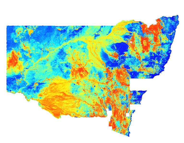
Pseudocolour image of the percentage of potassium (K%) in the upper 20 centimetres of the ground. Cooler colours indicate lower abundances of potassium and warmer colours represent higher abundances. Variations in potassium values are caused by varied mineral compositions in host rocks and soils. This statewide image was generated by merging many individual airborne radiometric surveys.
-

Depth to the Mohorovičić discontinuity (Moho) interpreted and modelled by Geognostics with support from government and industry. The Moho surface is the boundary between the Earth's crust and the upper mantle. The depth to moho is a representation of the thickness of the Earth's Crust. This moho surface is derived from seismic, gravity and other geophysical datasets.