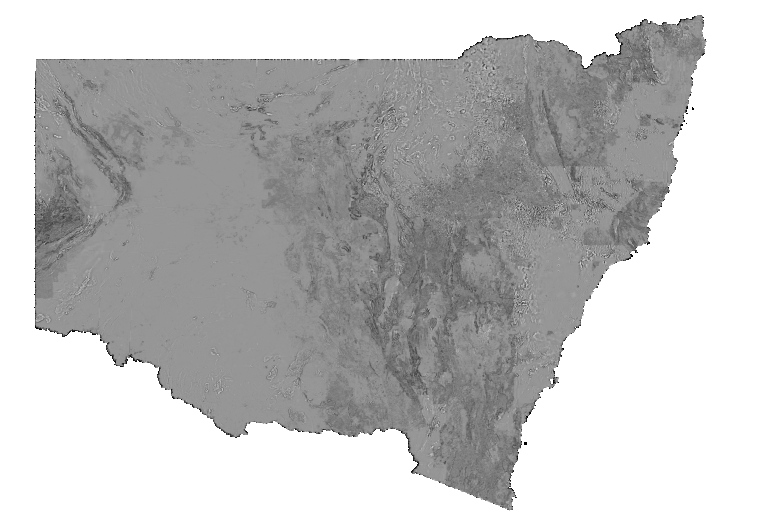
NSW Second Vertical Derivative of TMI RTP (2VD TMI RTP)
Greyscale image of second vertical derivative (2VD) of total magnetic intensity reduced to the pole (TMI RTP). Darker tones indicate lower values and lighter tones represent higher values. Reduction to the pole filters magnetic anomalies to appear as if the Earth's magnetic field were locally vertical, as at the magnetic pole (assuming all magnetic sources are inductively magnetised). The 2VD filter shows the vertical rate of change in the first vertical derivative (1VD) of the Earth's total magnetic field and enhances boundaries and structural detail of shallow sources further than 1VD. The 2VD filter enhances magnetic textures in the image, however, it also amplifies non-geological noise. Variations in the magnetic field are caused by lithological factors, principally magnetite (and/or pyrrhotite) content. This Statewide image was generated by merging many individual airborne magnetic surveys.
Simple
Identification info
- Date (Revision)
- 2024-05-06
- Status
- Completed
- Topic category
-
- Geoscientific information
- Keywords (Theme)
-
- Geophysics
- Magnetics
- 2nd Derivative
- Keywords (Place)
-
- New South Wales
- Language
- English
Distribution Information
- Distribution format
-
- Web Map Service
Distributor
- OnLine resource
- DIGS product page
- OnLine resource
- Download 2VD TMI RTP 2024 ERS file (4.5GB)
- OnLine resource
- Download 2VD TMI RTP 2024 TIF file
Resource lineage
- Statement
- Step 1 – QA/QC All available geophysics within the bounds of the state was assessed for quality. Poor data was remade or salvaged when and where available to do so. All metadata from each survey was harvested and compiled in a database. Step 2 – Quantify best available data An algorithm was created to aide in a quantitative assessment of which surveys were “better” than other surveys. This allowed for the decision of a lower bound to delineate which surveys were not of sufficient quality to be added to the merge. The algorithm utilised: • Line spacing • Ground clearance • Survey area • Sampling rate • Survey bearing relative to geological strike • Survey year Each of these aspects were provided a weighted score and input to the final equation to provide a final score. Line-Spacing / Clearance / Area / Sampling / Bearing / Year = Score It was discovered that a score of 100 was roughly equivalent to the data currently provided in the government-only statewide merge; therefore this became the cut-off for company data. Anything below a score of 100 was not of sufficient quality to add to the merge. Step 3 – Reproject and resample data All data for a merge must have the same grid cell size and the same projection. An extensive resampling/reprojection process was undertaken over both government and company data alike to unify the cell sizes. Two iterations of each survey were created: 50m, and 25m. Extensive notes on this process are maintained separate to this document. Step 4 – Determine precise layering An extensive vectorisation of all grids was performed to determine their precise locations of all survey boundaries and allow for assessment of all overlaps. Prior to the merge process it must be determined which overlapping surveys are of higher quality than each other. When possible, this was performed using the algorithmic score, however often it would be seen that two surveys shared the same score. In this case the decision was made manually based on the visual quality of the data. Where feasible, newer data was given preference. Step 5 – Clip and buffer the grids To achieve best results when merging grids, the area under the new addition should be blanked out of the base grid into which it is merged (excepting ~1000m overlap on edges). This therefore requires precise understanding of the outlines of the surveys being added to the merge. Using the layering determined in step 4, all underlying grids were clipped (with 500m external buffer) such that the only overlap remaining was on the edges of each boundary. Extensive notes on the exact layering and clipping process are maintained separate to this document. Step 6 – Perform the merge in multiple stages Stage 1: Rebuild government base layer from the ground up This was performed to ensure full control/understanding of the final product was available. • All government surveys were merged together and were tilt adjusted to the AWAGS2 line data • This first-pass merge was then merged with the existing pre-merged BMR data along the east coast of NSW using a surface adjust. The range and stretch of the BMR data was applied to the rest of the state to maintain continuity with the previous (2014) merge. Stage 2: Merge company data • The outlines for each company survey were clipped from the stage 1 merge for reasons outlined above. • All company data was merged into this grid using a surface adjust and maintaining the range and stretch from stage 1. Stage 3: Extensive QA/QC • The new merge was assessed extensively to ensure that no artefacts were being added to the grid by the company data dating back as far as the 1970s. • Several such artefacts were found and subsequently remedied. • Conversely it was discovered that some artefacts were present in the 2014 merge which were false and the high resolution company data shed new light on the areas. Step 7 – Filtering and reprojecting - RTP (nT) - 1VD (nT/m) - 2VD (nT/m) - RTP 1VD (nT/m) - RTP 2VD (nT/m) - RTP Tilt (degrees)
- Hierarchy level
- Dataset
Reference System Information
- Reference system identifier
- EPSG:3857
Reference System Information
- Reference system identifier
- CRS:84
Metadata
- Metadata identifier
- urn:uuid/dcbd5b9f-2bd5-48eb-a897-27c1a8440878
- Language
- English
- Character encoding
- UTF8
Type of resource
- Resource scope
- Dataset
- Metadata linkage
- https://geonetwork.geoscience.nsw.gov.au/geonetwork/srv/api/records/dcbd5b9f-2bd5-48eb-a897-27c1a8440878
- Date info (Revision)
- 2024-05-09T17:53:25
- Date info (Creation)
- 2020-11-19T09:10:59
Metadata standard
- Title
- ISO 19115:2003/19139
- Edition
- 1.0